OrthoNode
The OrthoNode class in Geomapi represents the data and metadata of Orthogonal Photos, often derived from photogrammetric reconstructions. The metadata builds upon the RDFlib framework:
https://rdflib.readthedocs.io/
The code below shows how to create a OrthoNode from various inputs.
First the geomapi and external packages are imported
#IMPORT PACKAGES
from rdflib import Graph
import os
import numpy as np

#IMPORT MODULES
from context import geomapi #context import for documentation only
from geomapi.nodes import OrthoNode
Jupyter environment detected. Enabling Open3D WebVisualizer.
[Open3D INFO] WebRTC GUI backend enabled.
[Open3D INFO] WebRTCWindowSystem: HTTP handshake server disabled.
OrthoNode Creation
A OrthoNode is constructed using the same parameters as the base Node. Please refer to Node Tutorial For more info about Node Creation
OrthoNode( subject = None,             # (URIRef, optional) : A subject to use as identifier for the Node.
          graph = None,               # (Graph, optional) : An RDF Graph to parse.
          graphPath = None,           # (Path, optional) : The path of an RDF Graph to parse.
          name = None,                # (str, optional) : A name of the Node.
          path = None,                # (Path, optional) : A filepath to a resource.
          timestamp = None,           # (str, optional) : Timestamp for the node.
          resource = None,            # (optional) : Resource associated with the node.
          cartesianTransform = None,  # (np.ndarray, optional) : The (4x4) transformation matrix.
          orientedBoundingBox = None, # (o3d.geometry.OrientedBoundingBox, optional) : The oriented bounding box of the node.
          convexHull = None,          # (o3d.geometry.TriangleMesh, optional) : The convex hull of the node.
          loadResource = False,       # Load the resource at initialization?
          dxfPath = None,             # (Path, Optional) : Path to the dxf file with the orthometadata from MetaShape.
          tfwPath = None,             # (Path, Optional) : Path to the tfw file with the orthometadata from MetaShape.
          imageWidth = None,          # (int, Optional) : width of the image in pixels (u). Defaults to 2000pix
          imageHeight = None,         # (int, Optional) : height of the image in pixels (v). Defaults to 1000pix
          gsd = None,                 # (float, Optional) : Ground Sampling Distance in meters. Defaults to 0.01m
          depth = None,               # (float, Optional) : Average depth of the image in meters. Defaults to 10m
          height = None               # (float, Optional) : Average height of the cameras that generated the image in meters.
        )
Ontology link
The OrthoNode has 7 new standard properties that are serialized to the graph:
python name |
predicate |
|---|---|
|
|
|
|
|
|
|
|
|
|
|
|
|
|
Creation From tfw file
OrthoNodes can be created from accompanying tfw files, these provide extra metadata like the gsd and cartesianTransform.
node = OrthoNode(tfwPath=r"../../../tests\testfiles\ortho\railway-0-0.tfw")
print(node.gsd)
print(node.cartesianTransform)
0.01560589037
[[ 1.00000000e+00  0.00000000e+00  0.00000000e+00  2.63379145e+05]
 [ 0.00000000e+00 -1.00000000e+00  0.00000000e+00  1.51097344e+05]
 [ 0.00000000e+00  0.00000000e+00 -1.00000000e+00  0.00000000e+00]
 [ 0.00000000e+00  0.00000000e+00  0.00000000e+00  1.00000000e+00]]
Creation From dxf file
OrthoNodes can be created from autocad dfx files.
Since dxf files contain a large amount of elements, they cannot be loaded directly into a OrthoNodes.
Use the geomapi.tools.dxf_to_ortho_nodes function to load all elements into a list of OrthoNode.
import geomapi.tools as tl

linesetnodes = tl.dxf_to_ortho_nodes(dxfPath = r"../../..\tests\testfiles\ortho\railway-scheme.dxf")
Reading DXF file from ..\..\..\tests\testfiles\ortho\railway-scheme.dxf...
Loaded 1 OrthoNodes from DXF.
OrthoNode Resource
When creating a Node with a resource, it can be done either directly with the resource, or with the path to the resource.
A resource can be a big piece of data, this is why it is not always wanted to load the whole resource at initialization. This is why the loadResource parameter is default to False
For more info on specific resources, see the corresponding Node type
Loading The Resource
node = OrthoNode(path=r"../../../tests\testfiles\ortho\railway-0-0.tif", loadResource=False)
print("resource before loading:",node.resource)
node.load_resource() # Use specialized node fo each type of resource.
print("resource after loading:",node.resource)
Resource not loaded, but path is defined, call `load_resource()` to access it.
Resource not loaded, but path is defined, call `load_resource()` to access it.
Resource not loaded, but path is defined, call `load_resource()` to access it.
resource before loading: None
resource after loading: [[[255 255 255]
  [255 255 255]
  [255 255 255]
  ...
  [255 255 255]
  [255 255 255]
  [255 255 255]]

 [[255 255 255]
  [255 255 255]
  [255 255 255]
  ...
  [255 255 255]
  [255 255 255]
  [255 255 255]]

 [[255 255 255]
  [255 255 255]
  [255 255 255]
  ...
  [255 255 255]
  [255 255 255]
  [255 255 255]]

 ...

 [[255 255 255]
  [255 255 255]
  [255 255 255]
  ...
  [ 90  87  80]
  [100  93  92]
  [ 88  80  79]]

 [[255 255 255]
  [255 255 255]
  [255 255 255]
  ...
  [ 97  90  85]
  [ 97  94  92]
  [ 92  90  83]]

 [[255 255 255]
  [255 255 255]
  [255 255 255]
  ...
  [ 89  83  81]
  [106 103 106]
  [ 92  86  83]]]
Saving The Resource
A Ortho resource can be saved to disk using the save_resource() function.
Currently supports: .ply, .obj
node = OrthoNode(path=r"../../../tests\testfiles\ortho\railway-0-0.tif", loadResource=True)
node.save_resource(directory=r"../../../tests/testfiles/resources", extension=".tif") # Save the resource to the resourcePath
True
OrthoNode Transformation
Since every nod has a cartesian transform, it can be transformed using the node.transform() function.
The transformation also updates the convexHull and orientedBoundingBox.
Furthermore, if the OrthoNode has a resource, that resource is also transformed.
node = OrthoNode()
print(node.cartesianTransform)
transformation = np.array([[0,0,1,0],[0,1,0,0],[1,0,0,0],[0,0,0,1]])
node.transform(transformation=transformation)
print("applying transformation: (-1)")
print(node.cartesianTransform,"\n")

node = OrthoNode()
rotation = np.array([90,0,0]) #eulers in degrees
node.transform(rotation=rotation)
print("applying rotation: (90,0,0)")
print(node.cartesianTransform,"\n")

node = OrthoNode()
translation = np.array([1,2,3])
node.transform(translation=translation)
print("applying translation: (1,2,3)")
print(node.cartesianTransform)
[[1. 0. 0. 0.]
 [0. 1. 0. 0.]
 [0. 0. 1. 0.]
 [0. 0. 0. 1.]]
applying transformation: (-1)
[[0. 0. 1. 0.]
 [0. 1. 0. 0.]
 [1. 0. 0. 0.]
 [0. 0. 0. 1.]]

applying rotation: (90,0,0)
[[ 1.000000e+00  0.000000e+00  0.000000e+00  0.000000e+00]
 [ 0.000000e+00  6.123234e-17 -1.000000e+00  0.000000e+00]
 [ 0.000000e+00  1.000000e+00  6.123234e-17  0.000000e+00]
 [ 0.000000e+00  0.000000e+00  0.000000e+00  1.000000e+00]]

applying translation: (1,2,3)
[[1. 0. 0. 1.]
 [0. 1. 0. 2.]
 [0. 0. 1. 3.]
 [0. 0. 0. 1.]]
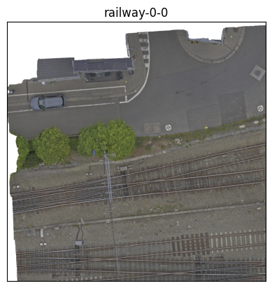
OrthoNode Visualisation
When a OrthoNode has a resource, the show() function displays the Orthophoto using PIL
node = OrthoNode(path=r"../../../tests\testfiles\ortho\railway-0-0.tif", loadResource=True)
node.show()
Further reading
Please refer to the full API documentation of the OrthoNode class for more details about the functionality